Analysis on the Arena of Hearthstone

Hearthstone is a game I play now and then. It’s a strategy card game, where you have different heroes, magic cards, monsters, etc; It’s fun game to play. Recently, my friend posted a picture of him receiving many rewards, because he won $12$ games in the arena in Hearthstone. This got me thinking, how likely does this event happen. Of course, It’s rare, which is certainly true to me(I’m not good at it). But depending on one’s skill, the likelihood will different. The reasoning is intuitively sound, but I want to do a more careful analysis on it.

Arena in Hearthstone is a place where you compete with players one at the time, with a deck you build from random cards. The arena is over when either you win $12$ games or lose $3$ games. Depending on the number of games of you stay in the arena, you will get different random generated awards. Of course, the longer you stay, the higher chance you get better awards. For someone like me, the chance is very bad; my best record is staying for $4$ games, which means I lost $3$ games out of $4$.

There are two ingredients for rare events like staying for $12$ games in the arena: skill and luck. Skill is relative, meaning it depends on the total skill levels in a pool of players. So I propose to quantify skill as the probability of winning a game, which can be interpreted as the percentage of the players that your skill is better than. the other factor is luck, which is the luck to stay for 12 games. I don’t have any comment about it, However I do want to point out that luck is sometimes we sort of know but don’t know exactly what it is. If you want a technical review about what is luck, or probability, you can read post from Terence Tao. Let me warn you: it’s very technical.

Let’s model the skill of a player as random variable $\boldsymbol\alpha$, and the number of total game play before lose $r$ games as $\mathbf X$. $\boldsymbol\alpha$ is a beta distribution. For a unknown player, we shall make it $\beta(1,1)$. $\mathbf X$ is binomial like distribution, which depends on two parameters $\boldsymbol\pi$ and $r$, and r is 3 in our case.

Here is the DAG(Directed Acyclic Graph) representation of the model: Since $\boldsymbol\alpha \sim \beta(1,1)$, $p(\boldsymbol\pi)$ is straight-forward, which is $1$. $p(\mathbf x| \boldsymbol\pi, r)$ requires a little work. Let’s first remove the constraint that a player can only stay up to 12 games, then:

If the constraint is relaxed, we need to transform the (1). The constraint that $\mathbf x \leq N$, means that events ${N,N+1..}$ is just one event, which let’s defined as N for mathematical convenience and intuitive reason(N is the maximum). then, we can rewrite (1) as:

Now we ready to obtain the joint probability function: $p(\boldsymbol\pi,\mathbf x) = p(\boldsymbol\pi)p(\mathbf x|\boldsymbol\pi, r)$. With parameters $N = 12$ and $r = 3$, we will have:

The equation $(2)$ is every thing we need to perform analysis. Let’s see what the model says about my friend’s skill based on that he stayed for $12$ games for one time, $p(\boldsymbol \pi | \mathbf x = 12)$: 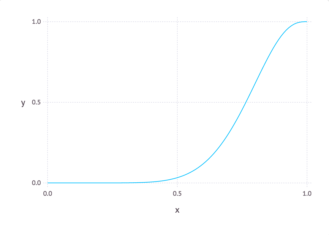This graph sort of matches with our intuition. Staying for $12$ games is not a easy thing, which probably means that my friend has higher skill than many other players.

Now let’s see what the model says about my skill. On average I stayed only for $4$ games: 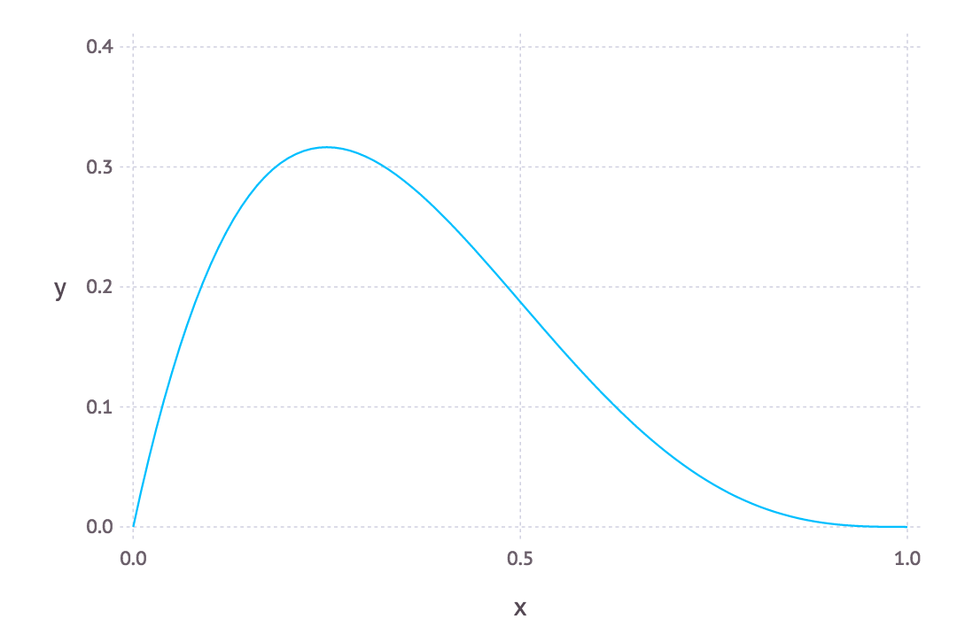The result was better than I thought. I thought it will be highly concentrated near $0$.

Some analysis from the model actually surprised me. For example, for high skill player, It’s much more likely to stay for $12$ games, than any other individual outcome, like $11$. $p(\mathbf x | \boldsymbol \pi = 0.8)$: 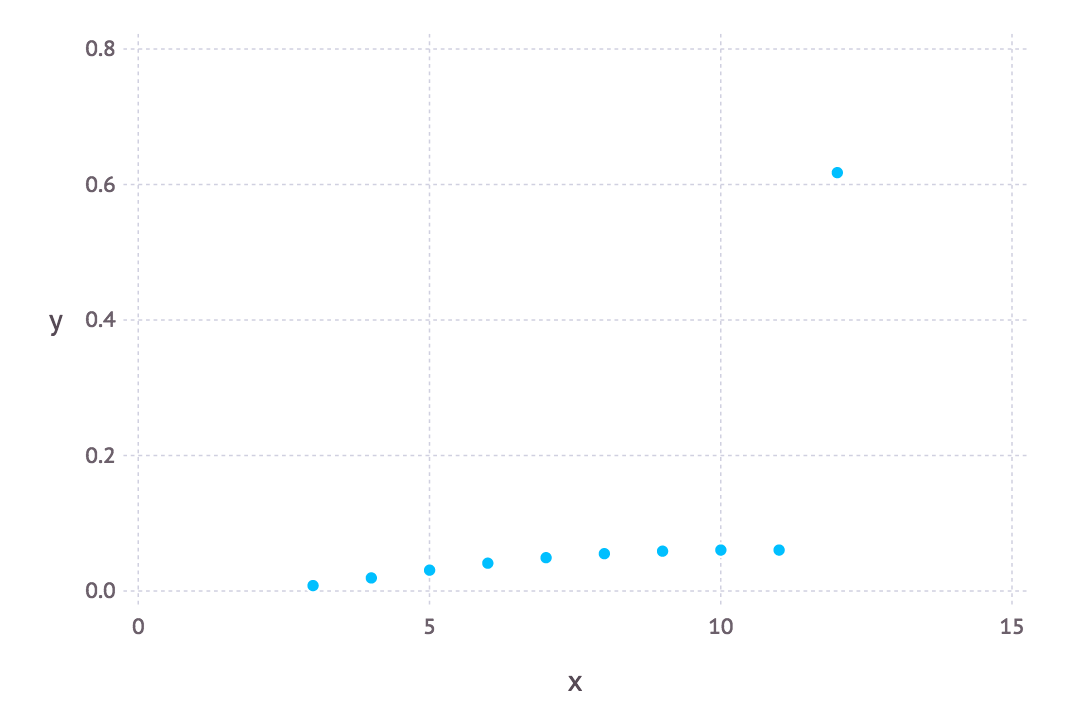But when you carefully think about it, It makes sense. Because for high skill player, the tail events has tangible probability, which has been summed up when the game stops at $12$.

There are some extra things I want to point out. In this analysis, I only use single data for the model. The model can be extended to describe many more data about a player’s performance, which will have richer and more accurate information reflecting about the player. The arena has other aspect, which is worthy analyzing as well, like average reward for a player based on his skill. This kind of analysis can be good for making better decision about whether or not play the arena(Of course, we don’t do that, we play it just for fun). To do that, the existing model can be reused. I imagine It will be more complicated and other tools need to be used for analysis, for example importance sampling and MCMC.

Here is the code I used for generating these plots, in case anyone wants to simulate. I used Juno IDE and Gadfly package:

using Gadfly

#condition on pi
pi = 0.8
p(x, pi) = factorial(x-1)/(factorial(x-3)*2)*pi^(x-3)*(1-pi)^3
x = [3:12]
y = map((x)->p(x,pi),x)
y[end] += 1-foldr(+,y)
plot(x=x, y=y)

mean = foldr(+, x.*y)

#condiion on x
#from 3 to 11
n = 4
x2 = [0:0.01:1]'
y2 = map((pi)->p(n,pi), x2)
plot(x=x2, y=y2, Geom.line)


#for 12
p_for12(pi)=1-foldr(+,map((x)->p(x,pi),[3:11]))
x3 = [0:0.01:1]'
y3 = map(p_for12, x3)
plot(x=x3, y=y3, Geom.line)