
Introduction to Decision Tree
2015/09/13Decision tree is a machine learning method for doing classifications or regressions. To me, the decision tree is an interesting method; It combines both computer science and mathematics to achieve learning. Advance methods have been built on the idea of decision tree, which have been proved useful in many kaggle competitions.
Decision tree can be thought as a structure that makes successive judgments until a final decision is reached. For example, the process of deciding if a person likes video games or not can be decided using a decision tree [1]:
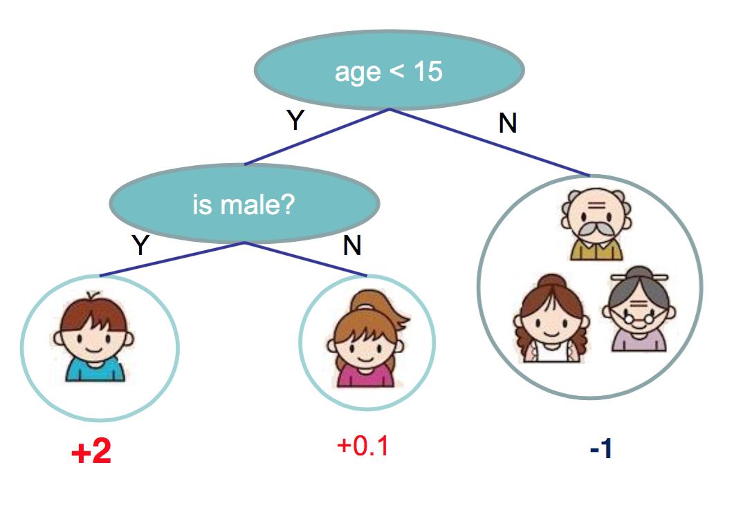
The leaf produces a number that indicates how likely does the person like video games. The higher the number is, the more likely it is. Let us go through the tree once. Suppose, we have a person who is male and is 12 years old. First, we check the age, and find out the person is less than 15. So we go to left. Next, we check what is the gender of the person, which is male in this case. So we will obtain 2.
As we can see, decision tree is a convenience structure for making decisions. But, how do we find such tree? In machine learning, we would like to search for the best tree given a data set, and use it to make predictions.
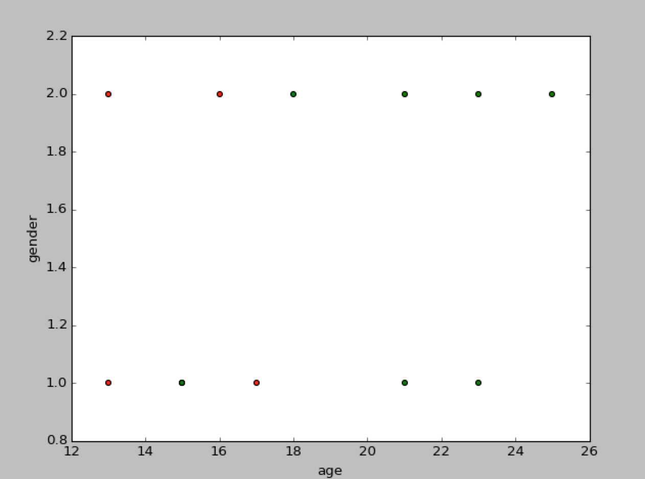
To better illustrate, we will use only computer generated data. For convenience, male and female will be represented by 1 and 2 respectively, and 1 represents the person likes video games, 0 otherwise.
| gender | age | like |
| 1 | 13 | 1 |
| 1 | 15 | 1 |
| 2 | 16 | 1 |
| 1 | 17 | 1 |
| 1 | 15 | 0 |
| 2 | 13 | 1 |
| 2 | 18 | 0 |
| 2 | 25 | 0 |
| 1 | 21 | 0 |
| 2 | 21 | 0 |
| 1 | 23 | 0 |
| 2 | 23 | 0 |
Of course, just by looking at numbers, we would be clueless about the data. Let us visualize it to get a sense of it(red means like, green mean dislike),
To construct the tree, the general idea is that we partition the data-set successively and obtain the best one. One way to do that is just use brute force; find all partitions and compare them to obtain the best one. But, the brute force is computationally infeasible, so we would use greedy search instead. The basic algorithm is simple: given a data-set, we pick a feature and a separate point that minimizes some loss function, then we recursively apply the same algorithm to the two partitioned data-set, until a stop point is met. For example, for our generated data-set, by using our vision inspection, we might want to first partition the data-set at age=18. Then we are going to partition the left and right partitioned data-sets with same fashion. One possible realization could be:
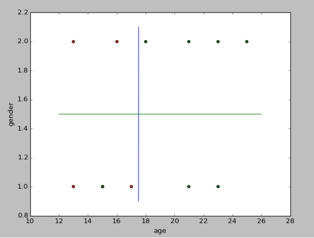
In this decision tree, if the person falls in the left top and left down region, we would say that he or she likes the video game, otherwise he or she does not like it.
Now let us fill some details about the algorithm. Let $D$ denote a data-set, $x := x_1,x_2,…x_N$ denote a feature vector, and $y$ denote the labels. In our case, $D$ would be the data-set consist of gender and age($x_1, x_2)$, and $y$ would be the vector of likes and dislike. Let $Q(\bullet)$ denote that the loss function given a data-set. let $D_l(j,s)$ be $\{x\}$ such that $x_j < s$, and $D_r(j,s)$ be $\{x\}$ such that $x_j \geqslant s$. Find the best separated point and the feature can be expressed as
\begin{equation} \min_{j,s} (Q(D_l(j,s))+Q(D_r(j,s))) \end{equation}
There are different $Q(\bullet)$ loss function we can choose, for example Gini index and Cross-entropy [2 9.17]. Note that we also need a stop point, otherwise, the algorithm would just keep partitioning. The simple way is just limit the depth of the tree.
The decision tree itself is not useful; It is prone to overfit the data. To deal with it, a process called pruning is used. The pruning removes unnecessary nodes according to the cost complexity criterion [2 9.16].
To conclude this, I will add a draft implementation of decision tree in Julia:
#pick_spoint implements the equation (1)
function build_tree(matrix, labels, depth, meta::Dict)
    if depth > meta["maxdepth"] || all(x->x==labels[1], labels)
        return Leaf(get_pk(labels,meta))
    else
        featid,spoint = pick_spoint(matrix, labels, meta)
        t = matrix[:,featid] .< spoint
        m_left,m_right = matrix[t,:],matrix[!t,:]
        l_left,l_right = labels[t], labels[!t]
        left_node = build_tree(m_left, l_left, depth+1, meta)
        right_node = build_tree(m_right, l_right, depth+1, meta)
        return Node(featid, spoint, get_pk(labels, meta), left_node, right_node)
    end
end
Note that, the recursion is very bad idea in terms of memory usage. Use for loop to do it is recommended, if the data-set is big.
reference:
[1]. Introduction to Boosted Trees, Tianqi Chen, 10 22 2014.
[2]. Hastie, T.; Tibshirani, R. & Friedman, J.(2001), The Elements of Statistical Learning, Springer New York Inc., New York, NY, USA.