Regression in Julia

Regression is the most basic tool in statistics and machine learning. Before many advancements of machine learning research, the regression was basically what everyone was doing; It is simple and yet very useful.

Even though Julia is in heavy developing phase, It already has serveral packages for doing regression. One of them is Regression. the Regression provides two inferfaces: high-level and low-level interface. I found low-level interface actually more straight-forward to use. Basically, there are two steps to follow. First, we formulate a prediction model with a loss function and possibly a regularizer, and then we pass it to a solver to obtain the values of parameters.

In the first part, basically we are formulating the equation,

\begin{equation} \sum_{i=1}^{n} loss(f(x_i;\theta),y_i)+r(\theta) \end{equation}

In $(1)$, there are three components: prediction model, loss function, and regularizer. Each of the components is from the EmpiricalRisks. With these components, we can construct the type of regression we want to have. After the selecting components, we glue them together with data to form (1).

In the second part, our objective is to minimizing (1). The minimization will gives us the optimal $\theta$ of our prediction model. There are several solvers we can pick to carray out the minimization, for example gradient descent, BFGS Quasi-Newton method etc, which can be found in the Regression package itself.

Let us see an example. Consider linear model with $n$ features, we will have following model:

\begin{equation} f(x;\theta) = \theta^Tx \end{equation}

then we can have a square loss function,

\begin{equation} loss(u,y) = \frac{1}{2}(u-y)^2 \end{equation}

Put togehter (2) and (3) we will have,

\begin{equation} loss(x,y) = \frac{1}{2}(\theta^Tx-y)^2 \end{equation}

We can also provide a regularizer to prevent overfitting or selecting features. The code for express these components,

using Regression
dim = 6                      # feature vector with n dimension
model = LinearPred(dim)      # the equatin (2)
sqrloss = SqrLoss()          # the loss function (3)
reg = SqrL2Reg(2.0)          # squared L2 regularizer with coefficient 1

Next, we put them together with the data to obtain the final form (1)

# this is (4)
rmodel = riskmodel(model,sqrloss)
# assume xs is the m by 6 matrix(list of feature vectors)
# and the ys is a vector of labels either -1 or 1
objective_function = Regression.RegRiskFun(rmodel, reg, xs', ys)

Note that, we only specify one loss function, and the final form of loss function is the sum of individual loss function. Are we mising something? The answer is no, This is because one loss function already contains enough information needed for the final form. For example, derivative of final form will be sum of each individual loss function. Each derivative of loss functions can be evaluated seperately with the data to get derivative of the final form.

Now we are ready to obtain the $\theta$,

# what we want to estimate
thetas = ones(Float64, dim)
# some adjustable parameters for optimization
options = Regression.Options()
# use gradient descent
solver = Regression.GD()
# run the optimization
Regression.solve!(solver, objective_function, thetas, options, Regression.no_op)

The function solve! has several parameters. Some of them can are used to customize the optimization, such as maximum number of iterations, converging threshold e.t.c. These details can be found on the README of the github repo.

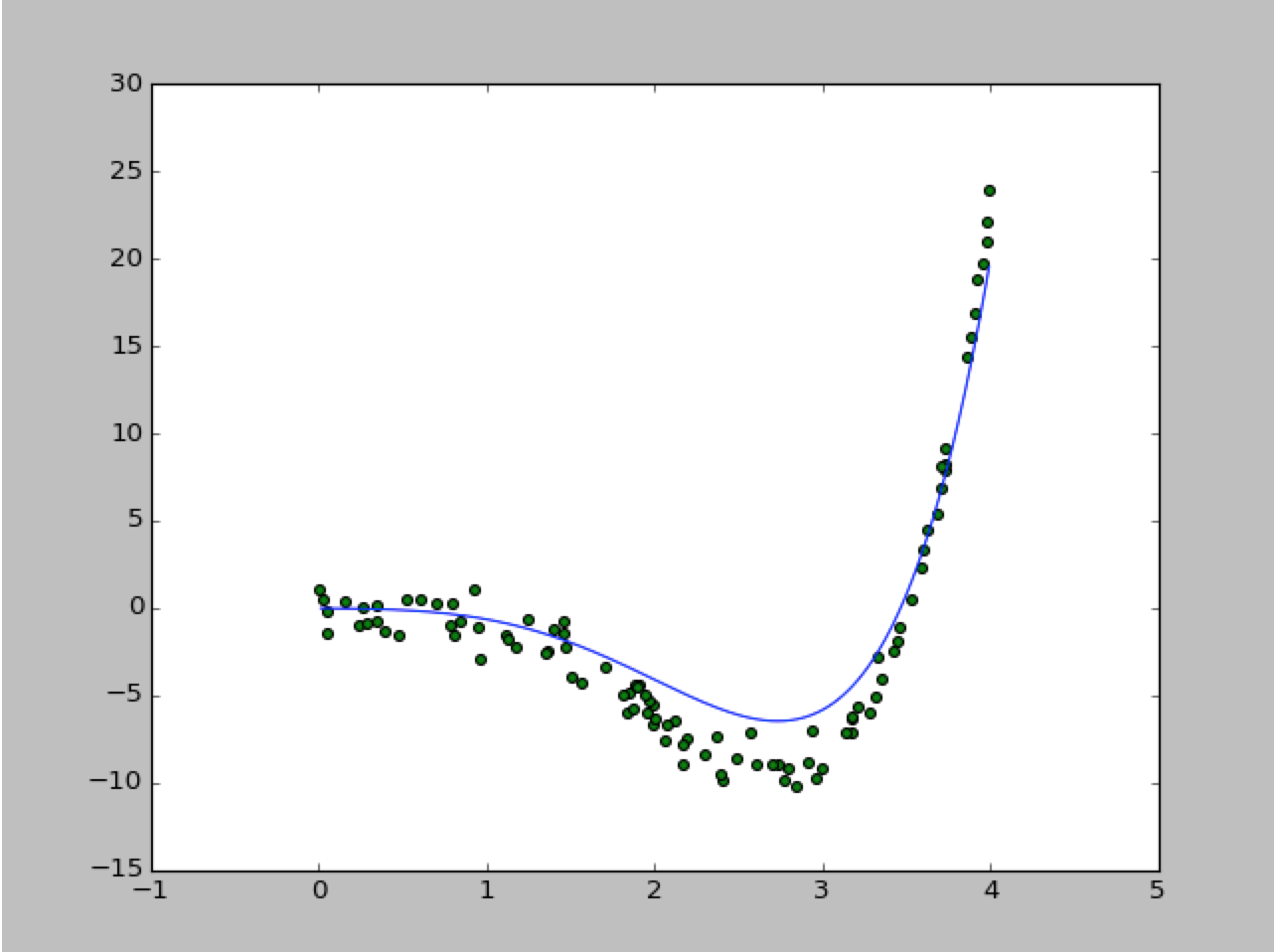
The simulation result,

If you want to play with the source code, click on here.